
Recently, I scraped data analyst job roles in Canada from Indeed and Glassdoor. The raw dataset was messy, and needed a thorough cleaning to make it analysis ready. In this tutorial, I'll be showing you complete start to end data cleaning process I performed.
Please refer to AI tools or Google if you want to understand full depth working of different functions and methods used, since I'll be displaying you code execution with output and basic explanations only.
To start, let us import required libraries and raw dataset. You can follow along me by downloading the raw dataset from Kaggle.
Image by freepikBasic Data Analysis 📝
import pandas as pd
import re
import numpy as np
import matplotlib.pyplot as plt
from wordcloud import WordCloud
from collections import Counter
from sklearn.feature_extraction.text import TfidfVectorizer
from sklearn.cluster import KMeans
from sklearn.metrics import silhouette_score
import matplotlib.pyplot as plt
from scipy.spatial.distance import cdist
from kneed import KneeLocator
df = pd.read_csv('./input/data-analyst-job-roles-in-canada/Raw_Dataset.csv')
# I like to make a copy of the original dataframe, and work on it.
dfCopy = df
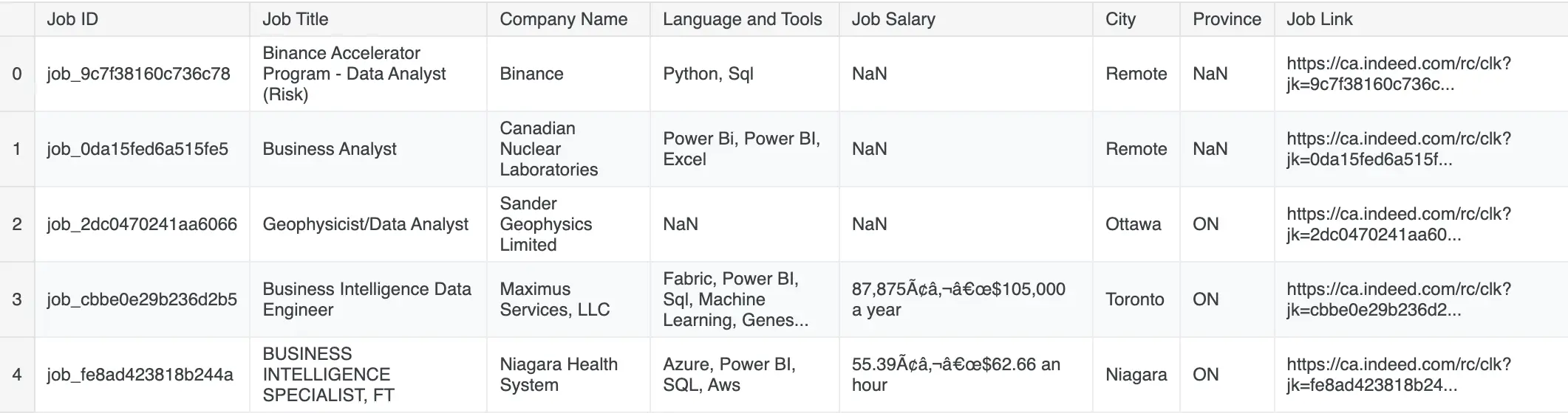
dfCopy.head(5)Output:
We can notice the Job ID and Job Link won't play significant role in data analysis, so we drop them.
# Dropping the Job ID and Job Link columns
# You can use inplace = True or assign it to the dataframe because
# drop() method does not modify the DataFrame in place by default.
# Instead, it returns a new DataFrame with the specified columns dropped.
dfCopy = dfCopy.drop(columns = ['Job ID','Job Link'])
The output of df.info() provides a concise summary of the DataFrame.
# There are 1796 row entries
# Columns are object datatypes
dfCopy.info()

# Output for info()

<class 'pandas.core.frame.DataFrame'>
RangeIndex: 1796 entries, 0 to 1795
Data columns (total 6 columns):
 #   Column              Non-Null Count  Dtype
---  ------              --------------  -----
 0   Job Title           1796 non-null   object
 1   Company Name        1796 non-null   object
 2   Language and Tools  1629 non-null   object
 3   Job Salary          1239 non-null   object
 4   City                1796 non-null   object
 5   Province            1678 non-null   object
dtypes: object(6)
memory usage: 84.3+ KB
Let us rename columns for easy recognition.
dfCopy = dfCopy.rename(columns={
    'Job Title': 'Position',
    'Company Name': 'Company',
    'Language and Tools': 'Skill',
    'Job Salary' : 'Salary',
})
Let us check for NULL values
dfCopy.isnull().sum()

# Output for NULL value checking

Position      0
Company       0
Skill       167
Salary      557
City          0
Province    118
dtype: int64
Treating NULL Values 🤫
We noticed columns 'Skill', 'Salary' and 'Province' has null values.
We can't add random values to 'Skill' columns, so we add 'Undef' to null. Similar, is the case with 'Province' column.
However, 'Salary' column can be adjusted and also we have 1/4th of values as NULL.
Let us just add some values to empty cells, we will deal with 'Salary' in a moment.
# Fill missing Province and Lang & tools values with a default value
dfCopy.fillna({'Skill': 'Undef', 'Province' : 'Undef', 'Salary' : 'Undef'}, inplace = True)
Let us confirm we fixed "NULL value issues" as of now.
# Rechecking for NULL values
dfCopy.isnull().sum()

# Output for above code

Position    0
Company     0
Skill       0
Salary      0
City        0
Province    0
dtype: int64
Great!
Let us start Cleaning the Data 🔎
Working with 'Position' column
unique_count = dfCopy['Position'].nunique()
print(f"Number of unique job positions : {unique_count}")

# Output : Number of unique job positions : 811
We need more generic role title in order to identify top jobs.
Let us use Clustering approach to group similar items together.
Basic idea: We will use Glove Embeddings to convert job titles into vectors and find optimal number of clusters by using Elbow, Gap Statistic and Silhouette method.
# Step 1: Preprocess the job titles
def preprocess_title(title):
    """
    Convert title to lowercase and remove punctuation.
    """
    title = title.lower()
    title = re.sub(r'[^\w\s]', '', title)  # Remove punctuation
    return title

# Apply preprocessing to 'Position'
dfCopy['Refined Title'] = dfCopy['Position'].apply(preprocess_title)

# Step 2: Load GloVe embeddings
def load_glove_embeddings(file_path):
    """
    Load GloVe embeddings from a file into a dictionary.
    """
    embeddings = {}
    with open(file_path, 'r', encoding='utf-8') as f:
        for line in f:
            values = line.split()
            word = values[0]
            vector = np.asarray(values[1:], dtype='float32')
            embeddings[word] = vector
    return embeddings

# Load GloVe embeddings (50-dimensional vectors in this case)
glove_file_path = './input/glove-embedding/glove.6B.50d.txt'
glove_embeddings = load_glove_embeddings(glove_file_path)

# Convert text to vectors using GloVe
def text_to_vector(text, embeddings):
    """
    Convert text into a vector by averaging GloVe vectors of its words.
    """
    words = text.split()
    vectors = [embeddings.get(word, np.zeros(len(next(iter(embeddings.values()))))) for word in words]
    return np.mean(vectors, axis=0) if vectors else np.zeros(len(next(iter(embeddings.values()))))

# Transform job titles into vectors
dfCopy['Vector'] = dfCopy['Refined Title'].apply(lambda x: text_to_vector(x, glove_embeddings))
X = np.array(dfCopy['Vector'].tolist())

# Step 3: Determine the optimal number of clusters using the Elbow Method
inertia = []
for n_clusters in range(1, 11):  # Testing from 1 to 10 clusters
    kmeans = KMeans(n_clusters=n_clusters, random_state=42, n_init='auto')
    kmeans.fit(X)
    inertia.append(kmeans.inertia_)

# Plot the elbow curve
plt.figure(figsize=(10, 6))
plt.plot(range(1, 11), inertia, marker='o')
plt.xlabel('Number of Clusters')
plt.ylabel('Inertia')
plt.title('Elbow Method for Optimal Clusters')

# Apply KneeLocator to find the "knee" or "elbow"
kneedle = KneeLocator(range(1, 11), inertia, curve='convex', direction='decreasing')
elbow_optimal_clusters = kneedle.elbow

# Mark the elbow on the plot
plt.axvline(x=elbow_optimal_clusters, color='r', linestyle='--')
plt.scatter(elbow_optimal_clusters, inertia[elbow_optimal_clusters - 1], color='r', s=100, zorder=5)
plt.grid(True)
plt.show()


# Step 4: Determine the optimal number of clusters using the Silhouette Score
silhouette_scores = []
for n_clusters in range(2, 11):  # Testing from 2 to 10 clusters
    kmeans = KMeans(n_clusters=n_clusters, random_state=42, n_init='auto')
    clusters = kmeans.fit_predict(X)
    score = silhouette_score(X, clusters)
    silhouette_scores.append(score)

# Plot the silhouette scores
plt.figure(figsize=(10, 6))
plt.plot(range(2, 11), silhouette_scores, marker='o')
plt.xlabel('Number of Clusters')
plt.ylabel('Silhouette Score')
plt.title('Silhouette Score for Optimal Clusters')

# Determine the optimal number of clusters based on highest silhouette score
silhouette_optimal_clusters = np.argmax(silhouette_scores) + 2  # Adding 2 because range starts from 2

# Mark the optimal number of clusters on the plot
plt.scatter(silhouette_optimal_clusters, silhouette_scores[np.argmax(silhouette_scores)], color='r', s=100, zorder=5)
plt.grid(True)
plt.show()


# Step 5: Determine the optimal number of clusters using the Gap Statistic
def compute_gap_statistic(X, k_max=10, n_refs=10):
    """
    Compute the Gap Statistic for a range of cluster numbers.
    """
    gaps = []
    stds = []
    for k in range(1, k_max + 1):
        kmeans = KMeans(n_clusters=k, random_state=42, n_init='auto').fit(X)
        dispersion = np.sum(np.min(cdist(X, kmeans.cluster_centers_, 'euclidean'), axis=1))

        # Generate reference dispersion
        ref_disps = []
        for _ in range(n_refs):
            ref_points = np.random.uniform(low=np.min(X, axis=0), high=np.max(X, axis=0), size=X.shape)
            ref_dispersion = np.sum(np.min(cdist(ref_points, kmeans.cluster_centers_, 'euclidean'), axis=1))
            ref_disps.append(ref_dispersion)

        gap = np.mean(np.log(ref_disps)) - np.log(dispersion)
        gap_std = np.std(np.log(ref_disps))
        gaps.append(gap)
        stds.append(gap_std)

    return gaps, stds

gaps, stds = compute_gap_statistic(X)

# Plot the Gap Statistic
plt.figure(figsize=(10, 6))
plt.errorbar(range(1, 11), gaps, yerr=stds, fmt='-o')
plt.xlabel('Number of Clusters')
plt.ylabel('Gap Statistic')
plt.title('Gap Statistic for Optimal Clusters')

# Determine the optimal number of clusters based on highest gap statistic
gap_optimal_clusters = np.argmax(gaps) + 1  # Adding 1 because range starts from 1

# Mark the optimal number of clusters on the plot
plt.scatter(gap_optimal_clusters, gaps[np.argmax(gaps)], color='r', s=100, zorder=5)
plt.grid(True)
plt.show()

print("\n")
print("=================================================================")
print(f"Optimal number of clusters (Elbow Method): {elbow_optimal_clusters}")
print(f"Optimal number of clusters (Silhouette Score): {silhouette_optimal_clusters}")
print(f"Optimal number of clusters (Gap Statistic): {gap_optimal_clusters}")
print("=================================================================")
print("\n")
By running above code, we get optimal number of clusters for three methods respectively.
=================================================================
Optimal number of clusters (Elbow Method): 4
Optimal number of clusters (Silhouette Score): 10
Optimal number of clusters (Gap Statistic): 10
=================================================================
We set the optimal no. of clusters to 10.
Let us use KMeans Clustering to assign cluster number based on optimal cluster size.
import warnings
warnings.filterwarnings("ignore")

# Step 6: Apply KMeans with the chosen number of clusters
kmeans = KMeans(n_clusters=gap_optimal_clusters, random_state=42)
clusters1 = kmeans.fit_predict(X)
dfCopy['Cluster'] = clusters1

# Step 7: Analyze clusters
cluster_summary = dfCopy.groupby('Cluster')['Position'].apply(list)

# Let us print the dataframe
dfCopy.head(5)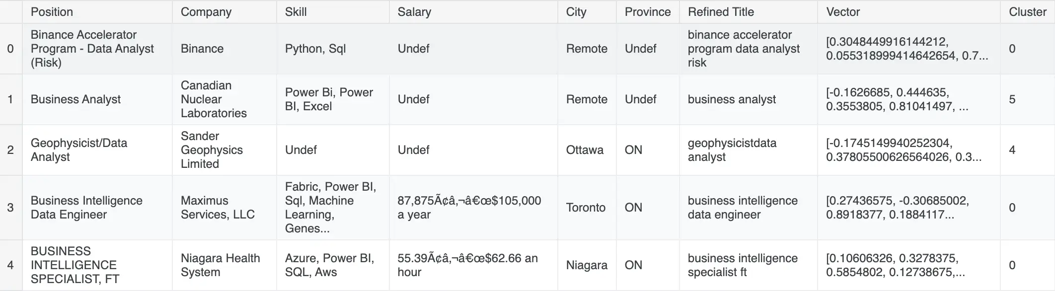
Visualizing the clusters to rename them using WordCloud.
# Get unique clusters and sort them
clusters = sorted(dfCopy['Cluster'].unique())

fig, axes = plt.subplots(nrows=5, ncols=2, figsize=(12, 25))
axes = axes.flatten()  # Flatten to make indexing easier

# Define a color map
color_map = plt.get_cmap('tab20', len(clusters))

# Loop through each cluster and create word clouds
for i, cluster in enumerate(clusters):
    # Filter titles for the current cluster
    cluster_text = ' '.join(dfCopy[dfCopy['Cluster'] == cluster]['Refined Title'])

    # Remove punctuation and non-alphanumeric characters
    cluster_text = re.sub(r'[^\w\s]', '', cluster_text)

    # Split text into words
    words = cluster_text.split()

    # Create a word frequency counter
    word_freq = Counter(words)

    # Create a WordCloud object
    wordcloud = WordCloud(width=800, height=400, background_color='white', colormap='tab20').generate_from_frequencies(word_freq)

    # Plot the word cloud
    ax = axes[i]
    ax.imshow(wordcloud, interpolation='bilinear')
    ax.axis('off')  # Hide the axes
    ax.set_title(f'Cluster {cluster}', fontsize=16)  # Increase font size for titles

# Remove empty subplots if there are fewer clusters than subplots
if len(clusters) < len(axes):
    for j in range(len(clusters), len(axes)):
        fig.delaxes(axes[j])

# Adjust layout for spacing
plt.tight_layout(pad=1.0, w_pad=10.0, h_pad=-50.0)  # Increase padding between plots

# Show plot
plt.show()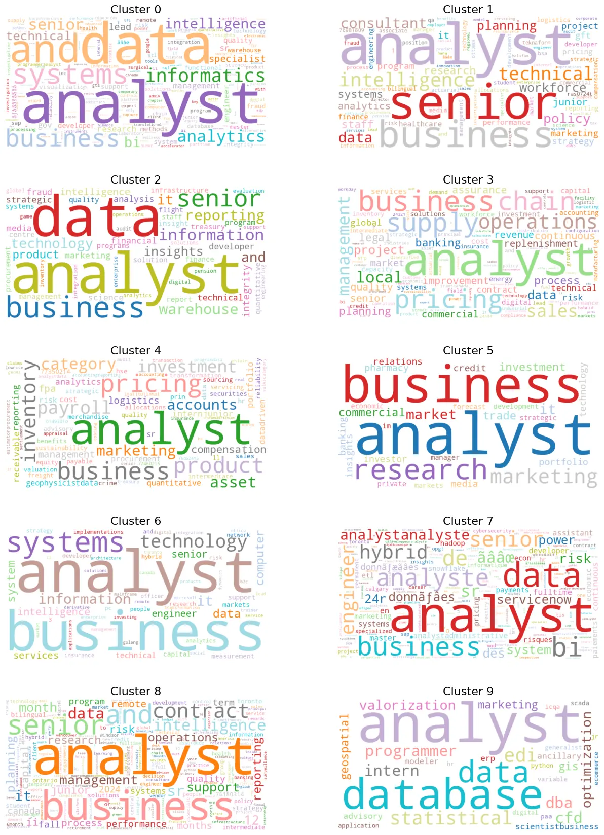
Cluster 0: Systems and Data Analysts Combines roles related to system analysis and data management.
Cluster 1: Senior Business Analysts Represents experienced professionals in business analysis.
Cluster 2: Business and Technical Analysts Features roles that blend business analysis with technical expertise.
Cluster 3 - Senior Supply Chain Data Analysts A specialist in analyzing business data within supply chain systems
Cluster 4: Financial and Operational Analysts Covers financial roles (pricing, payroll) and operational roles (inventory, quality assurance).
Cluster 5: Business and Marketing Analysts Includes roles in business analysis and marketing research.
Cluster 6: Business Systems Analysts Focused on improving and analyzing business systems and processes.
Cluster 7: Senior Data Analysts Experienced professionals who lead advanced data analysis efforts, providing insights and strategic recommendations.
Cluster 8: Senior Business Intelligence Analysts For senior roles focusing on data analysis and business intelligence.
Cluster 9: Database Analysts Specializes in managing and analyzing data within databases.
# Define the mapping of cluster values to job roles
cluster_to_job_title = {
    0: 'Systems and Data Analysts',
    1: 'Senior Business Analysts',
    2: 'Business and Technical Analysts',
    3: 'Senior Supply Chain Data Analysts',
    4: 'Financial and Operational Analysts',
    5: 'Business and Marketing Analysts',
    6: 'Business Systems Analysts',
    7: 'Senior Data Analysts',
    8: 'Senior Business Intelligence Analysts',
    9: 'Database Analysts'
}

# Create the new column with general job titles
dfCopy['Job Roles'] = dfCopy['Cluster'].map(cluster_to_job_title)

# Display the updated DataFrame
dfCopy.head(5)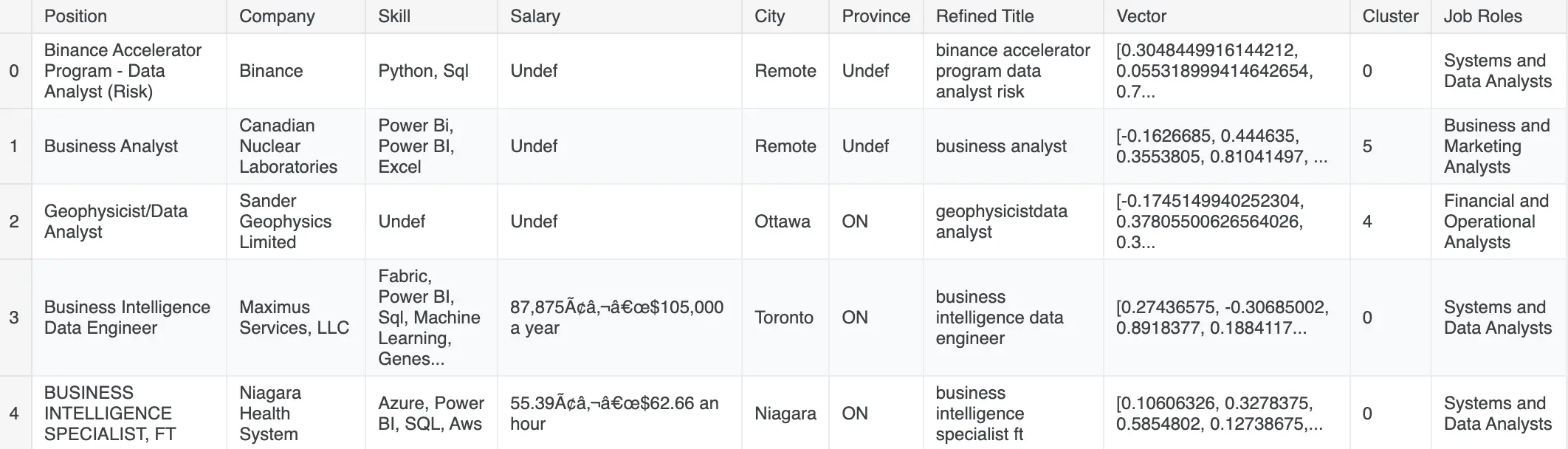
Lets create columns [Seniority, Position Type, Industry Type, Work Type]
Seniority Column
# Creating Seniority based on Job Title
# We are using regex because 'i','ii',... needs to be a separate words, not part of the word
def create_regex_patterns(keywords):
    """
    Create regex patterns with word boundaries for a list of keywords.
    """
    return [rf'\b{re.escape(keyword)}\b' for keyword in keywords]

def categorize_title(title):
    # Convert the title to lowercase for consistent comparison
    title_lower = title.lower()

    # Define keywords for each title level
    senior_keywords = ['senior', 'lead', 'principal', 'sr', 'iii', 'iv', 'senior level', 'advanced', 'senior associate','advance', 'expert', 'sr.', 'head', 'chief', 'director', 'manager', 'vp', 'specialist', 'mentor']
    mid_keywords = ['mid-level', 'mid level', 'midlevel', 'mid', 'ii', 'consultant', 'intermediate', 'experienced', 'associate', 'practitioner', 'level 2']
    junior_keywords = ['junior', 'entry level', 'intern', 'internship','apprentice', 'jr', 'i', 'jr.', 'assistant', 'beginner', 'trainee', 'novice', 'entry']

    # Create regex patterns
    senior_patterns = create_regex_patterns(senior_keywords)
    mid_patterns = create_regex_patterns(mid_keywords)
    junior_patterns = create_regex_patterns(junior_keywords)

    # Define the title levels and their patterns
    title_levels = [
        ('Senior', senior_patterns),
        ('Mid', mid_patterns),
        ('Junior', junior_patterns),
    ]

    # Iterate through the title levels and patterns to find a match
    for title_level, patterns in title_levels:
        if any(re.search(pattern, title_lower) for pattern in patterns):
            return title_level

    # Return 'ANY' if no patterns match
    return 'ANY'

# Apply the function to the 'Refined Title' column
dfCopy['Seniority'] = dfCopy['Refined Title'].apply(categorize_title)

# Print the DataFrame to verify
dfCopy[['Refined Title','Seniority']]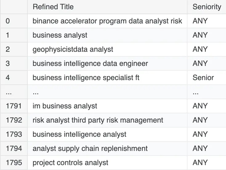
Position Type Column
# Creating Specific Job Positions
def categorize_title_types(title):
    # Convert the title to lowercase for case-insensitive matching
    title_lower = title.lower()

    # Define a list of title types with associated keywords
    title_types = [
        ('Developer', ['developer']),
        ('Programmer', ['programmer']),
        ('Data Specialist', ['specialist']),
        ('Writer', ['writer']),
        ('Manager', ['manager']),
        ('Data Consultant', ['consultant']),
        ('Coordinator', ['coordinator']),
        ('Technician', ['technician']),
        ('Administrator', ['administrator']),
        ('Admin', ['administrator']),
        ('Data Officer', ['officer']),
        ('Data Associate', ['associate']),
        ('Director', ['director']),
        ('Head', ['head']),
        ('Lead', ['lead']),
        ('Executive', ['executive']),
        ('Consultant', ['consultant']),
        ('Trainer', ['trainer']),
        ('Researcher', ['researcher']),
        ('Strategist', ['strategist']),
        ('Intern', ['intern']),
        ('Data Engineer', ['engineer']),
        ('Data Architect', ['architect']),
        ('Data Scientist', ['scientist']),
        ('Financial Analyst', ['financial analyst', 'finance']),
        ('Statistician', ['maths', 'mathematics', 'commerce']),
        ('Risk Analyst', ['risk analyst', 'risk']),
        ('Operation Analyst', ['Operation analyst', 'Operation']),
        ('Logistic Analyst', ['Logistic analyst','logistic']),
        ('System Analyst', ['Systems analyst', 'system']),
        ('Risk Analyst', ['risk analyst']),
        ('Quantitative Analyst', ['Quantitative Analyst','quantitative']),
        ('Business Analyst', ['business analyst']),
        ('BI Analyst', ['business intelligence analyst', 'business intelligence']),
        ('Data Analyst', ['data analyst']),
        ('Analyst', ['analyst']),
    ]

    # Iterate through the title types and keywords to find a match
    for position_type, keywords in title_types:
        if any(keyword in title_lower for keyword in keywords):
            return position_type

    # Default to 'Other' if no keywords match
    return 'Other'


# Apply the function to the 'Refined Title' column to create a new 'Position Type' column
dfCopy['Position Type'] = dfCopy['Refined Title'].apply(categorize_title_types)

# Print the DataFrame to verify
dfCopy[['Refined Title', 'Position Type']]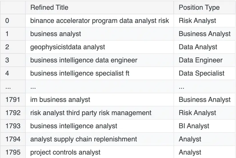
Work Type Column
# Type of Work - Remote, Hybrid, In-person
def categorize_work_type(title, city):
    # Convert both title and city to lowercase for case-insensitive matching
    title_lower = title.lower()
    city_lower = city.lower()

    # Define a list of work types with associated keywords
    work_types = [
        ('Remote', ['remote', 'work from home', 'wfh', 'telecommute', 'telework']),
        ('Hybrid', ['hybrid', 'partially remote', 'part-time remote', 'flexible']),
        ('In-Person', ['in-person', 'on-site', 'office', 'face-to-face', 'physical location'])
    ]

    # Check the work type keywords in both title and city simultaneously
    combined_text = f"{title_lower} {city_lower}"

    for work_type, keywords in work_types:
        if any(keyword in combined_text for keyword in keywords):
            return work_type

    # Default to 'In-Person' if no keywords match
    return 'In-Person'

# Apply the function to both 'Refined Title' and 'City' columns to create a new 'Work Type' column
dfCopy['Work Type'] = dfCopy.apply(lambda row: categorize_work_type(row['Refined Title'], row['City']), axis=1)

# Print the DataFrame to verify
dfCopy[['Refined Title', 'City', 'Work Type']]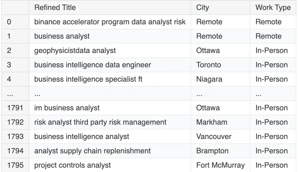
Industry Type Column
# Industry Type
def categorize_industry_type(company_name):
    # Convert company name to lowercase for case-insensitive matching
    company_name_lower = company_name.lower()

    # Define a list of industries with associated keywords
    industry_types = [
    ('Technology', ['tech', 'information', 'software', 'hardware', 'it', 'information technology', 'computing', 'digital','foilcon']),
    ('Finance', ['finance', 'bank', 'investment', 'financial', 'credit', 'securities', 'capital']),
    ('Healthcare', ['healthcare', 'hospital', 'medical', 'pharma', 'biotech', 'med', 'clinic','island health', 'health','cancer']),
    ('Retail', ['retail', 'store', 'shop', 'e-commerce', 'merchant', 'outlet', 'shopping']),
    ('Education', ['education', 'university', 'school', 'college', 'academy', 'institute', 'learning']),
    ('Manufacturing', ['manufacturing', 'factory', 'production', 'plant', 'assembly', 'industrial']),
    ('Telecommunications', ['telecom', 'communication', 'network', 'wireless', 'cellular', 'broadband']),
    ('Energy', ['energy', 'oil', 'gas', 'renewables', 'electric', 'power', 'utilities']),
    ('Consulting', ['consulting', 'advisor', 'consultant', 'advisory', 'strategy', 'solutions']),
    ('Transportation', ['transportation', 'logistic', 'shipping', 'aviation', 'freight', 'delivery']),
    ('Insurance', ['insurance', 'underwriting', 'risk', 'policy', 'coverage']),
    ('Service', ['service', 'services', 'support', 'maintenance', 'facility']),
    ('Government', ['county', 'city', 'state', 'federal', 'municipal', 'government']),
    ('Real Estate', ['real estate', 'property', 'brokerage', 'land', 'estate']),
    ('Legal', ['legal', 'law', 'attorney', 'firm', 'litigation', 'legal services']),
    ('Media', ['media', 'broadcast', 'publishing', 'entertainment', 'press']),
    ('Agriculture', ['agriculture', 'farming', 'agri', 'horticulture', 'crop']),
    ('Automotive', ['automotive', 'car', 'vehicle', 'automobile', 'motor']),
    ('Construction', ['construction', 'builder', 'contractor', 'engineering', 'development']),
    ('Travel', ['travel', 'tourism', 'hospitality', 'resort', 'tour']),
    ('Aerospace', ['aerospace', 'aviation', 'space', 'aircraft', 'defense'])
    ]

    # Iterate through the industry types and keywords to find a match
    for industry_type, keywords in industry_types:
        if any(keyword in company_name_lower for keyword in keywords):
            return industry_type

    # Default to 'Other' if no keywords match
    return 'Others'

# Apply the function to the 'Company Name' column to create a new 'Industry Type' column
dfCopy['Industry Type'] = dfCopy['Company'].apply(categorize_industry_type)

# Print the DataFrame to verify
dfCopy.head()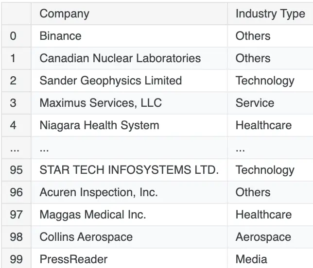
Let us check the info() to analyze our dataset.
dfCopy.info()

# Output for info()

<class 'pandas.core.frame.DataFrame'>
RangeIndex: 1796 entries, 0 to 1795
Data columns (total 14 columns):
 #   Column         Non-Null Count  Dtype
---  ------         --------------  -----
 0   Position       1796 non-null   object
 1   Company        1796 non-null   object
 2   Skill          1796 non-null   object
 3   Salary         1796 non-null   object
 4   City           1796 non-null   object
 5   Province       1796 non-null   object
 6   Refined Title  1796 non-null   object
 7   Vector         1796 non-null   object
 8   Cluster        1796 non-null   int32
 9   Job Roles      1796 non-null   object
 10  Seniority      1796 non-null   object
 11  Position Type  1796 non-null   object
 12  Work Type      1796 non-null   object
 13  Industry Type  1796 non-null   object
dtypes: int32(1), object(13)
memory usage: 189.5+ KB
Working with Salary Column 💰
Let us check the content of Salary column.
dfCopy['Salary']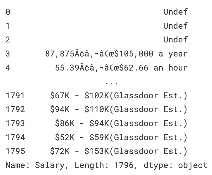
It is a real messy column. Let us start by analyzing what all characters are present in Salary column.
Cleaning Unncessary Characters from Salary column
# Concatenate all non-digit characters into a single string
non_digit_string = ''.join(dfCopy['Salary'].str.replace(r'\d+', '', regex=True).tolist())
# Convert to a set to get unique characters and then back to a string
unique_non_digit_string = ''.join(sorted(set(non_digit_string)))
print(unique_non_digit_string)
# Output for unique_non_digit_string
$&()*+,-./:;ABCDEFGHIJKLMNOPRSTUVWYabcdefghiklmnopqrstuvwxyz ¢¬ÂÃ✚ƒ‚€#Let us remove all characters we do not need, we create a function clean_salary() that filters unnecessary characters. It is important to analyze Salary column more to find out salary values are distributed.
# Function to clean the 'Salary' column
def clean_salary(text):
    if pd.notnull(text):  # Check if the text is not null
        # Replace characters not in the allowed patterns with an empty string
        # If we analyze, Glassdoor has unique 'K' character attached to values, lets convert that to number
        thousand_text = re.sub(r'(\d+)\s*K\b', lambda m: str(int(m.group(1)) * 1000), text)
        # Remove the parentheses
        text_no_parentheses = re.sub(r'\(.*?\)', '', thousand_text)
        # Remove everything except: digits, hour, year, undef, annual, day, - , ‚
        # Just a reminder: The character ‚ is not a comma
        cleaned_text = re.sub(r'[^\d‚\-\s.\b(hour|year|annual|day|Undef)\b]*', '', text_no_parentheses)
        return cleaned_text
    return ''  # Return an empty string if the text is null

# Apply the function to the 'Salary' column
dfCopy['Refined Salary'] = dfCopy['Salary'].apply(clean_salary)


dfCopy[['Salary','Refined Salary']]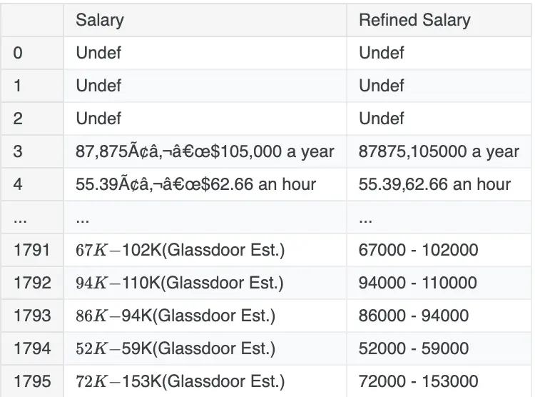
Now, we know how salary is distributed, we might need to convert all salaries into per year rate, and also we will divide them into Min & Max salaries, later we calculate Avg salary once we fix outliers.
# Lets again analyze the characters present in our Salary Column after refining
# Concatenate all non-digit characters into a single string
non_digit_string = ''.join(dfCopy['Refined Salary'].str.replace(r'\d+', '', regex=True).tolist())

# Convert to a set to get unique characters and then back to a string
unique_non_digit_string = ''.join(sorted(set(non_digit_string)))

# Print the unique non-digit characters
print(unique_non_digit_string)

# Output for unique_non_digit_string

()-.Uadefhlnoruy ,
Creating Min and Max Salaries
# Create Minimum and Maximum Salary column.
def extract_salaries(salary_text):
    # Find all digit values separated by '‚', '-' or spaces
    matches = re.findall(r'\d+(?:\.\d+)?', salary_text)
    if matches:
        # Convert to float and get the first two values
        numbers = [float(match) for match in matches[:2]]
        # Checking if two separate values are present
        if len(numbers) == 2:
            min_salary, max_salary = numbers
            return min_salary, max_salary
        elif len(numbers) == 1:
            return numbers[0], numbers[0]  # Only one value
    return None, None

# Generalize all salaries to per year
def convert_to_yearly(min_salary, max_salary, salary_text):
    if 'hour' in salary_text:
        # Assuming 2080 work hours per year
        min_salary *= 2080
        max_salary *= 2080
    return min_salary, max_salary


# Apply the extraction function and create new columns
dfCopy[['Min_Salary', 'Max_Salary']] = dfCopy['Refined Salary'].apply(lambda x: pd.Series(extract_salaries(x)))

# Convert to numeric, forcing errors to NaN
dfCopy['Min_Salary'] = pd.to_numeric(dfCopy['Min_Salary'], errors='coerce')
dfCopy['Max_Salary'] = pd.to_numeric(dfCopy['Max_Salary'], errors='coerce')

# Convert to yearly salaries and calculate average
dfCopy[['Min_Salary', 'Max_Salary']] = dfCopy.apply(lambda row: pd.Series(convert_to_yearly(row['Min_Salary'], row['Max_Salary'], row['Refined Salary'])), axis=1)

# Print the DataFrame with relevant columns
dfCopy[['Refined Salary', 'Min_Salary', 'Max_Salary']]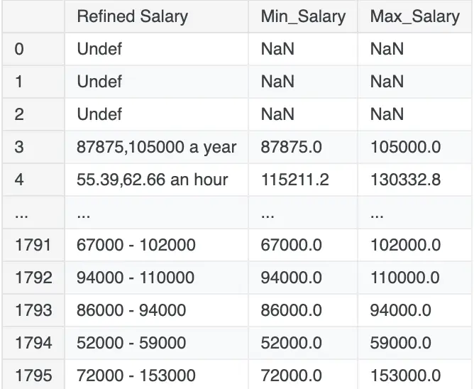
print(dfCopy[['Min_Salary', 'Max_Salary']].isna().sum())

# Output

Min_Salary    574
Max_Salary    574
dtype: int64
Data Imputation
Please read comments on the code for better understanding.
# Solving Missing values based on clusters
# Function to impute missing values based on cluster
def impute_missing_by_cluster(df, salary_col):
    # Group by Cluster and calculate the median salary for each cluster
    median_salaries = df.groupby('Cluster')[salary_col].median()

    # Define a function to fill missing values based on cluster
    def fill_missing(row):
        if pd.isna(row[salary_col]):
            return median_salaries[row['Cluster']]
        else:
            return row[salary_col]

    # Apply the function to the DataFrame
    df[salary_col] = df.apply(fill_missing, axis=1)

# Impute missing values for Min_Salary and Max_Salary based on cluster
impute_missing_by_cluster(dfCopy, 'Min_Salary')
impute_missing_by_cluster(dfCopy, 'Max_Salary')

dfCopy.isnull().sum()

# Output

Position          0
Company           0
Skill             0
Salary            0
City              0
Province          0
Refined Title     0
Vector            0
Cluster           0
Job Roles         0
Seniority         0
Position Type     0
Work Type         0
Industry Type     0
Refined Salary    0
Min_Salary        0
Max_Salary        0
dtype: int64
Checking Outliers in Min and Max Salary Columns
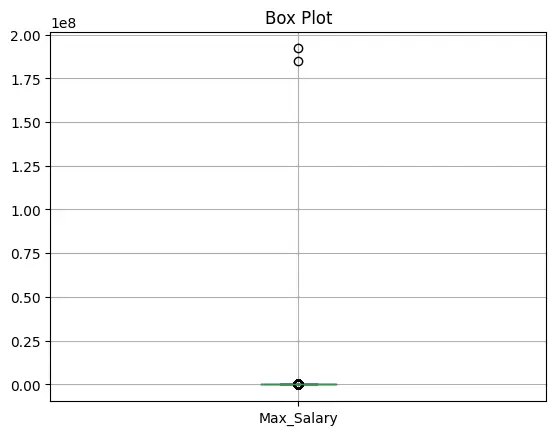
# Check minimum and maximum values in 'Min_Salary' & 'Max_Salary' column
min_avg_salary = dfCopy['Min_Salary'].min()
max_avg_salary = dfCopy['Min_Salary'].max()

min_max_salary = dfCopy['Max_Salary'].min()
max_max_salary = dfCopy['Max_Salary'].max()

print("Min Salary")
print(f"Minimum : {min_avg_salary}")
print(f"Maximum : {max_avg_salary}")
print("\n")
print("Max Salary")
print(f"Minimum : {min_max_salary}")
print(f"Maximum : {max_max_salary}")

# Output for above code

Min Salary
Minimum : 0.0
Maximum : 138661120.0


Max Salary
Minimum : 0.0
Maximum : 192098400.0
The difference is huge, lets find Q1,Q3, IQR and plot box plot to analyze the outliers.
# Calculate IQR for Min_Salary
Q1_min = round(dfCopy['Min_Salary'].quantile(0.25), 2)
Q3_min = round(dfCopy['Min_Salary'].quantile(0.75), 2)
IQR_min = round(Q3_min - Q1_min, 2)

# Determine outlier bounds for Min_Salary
lower_bound_min = round(Q1_min - 1.5 * IQR_min, 2)
upper_bound_min = round(Q3_min + 1.5 * IQR_min, 2)

# Calculate IQR for Max_Salary
Q1_max = round(dfCopy['Max_Salary'].quantile(0.25), 2)
Q3_max = round(dfCopy['Max_Salary'].quantile(0.75), 2)
IQR_max = round(Q3_max - Q1_max, 2)

# Determine outlier bounds for Max_Salary
lower_bound_max = round(Q1_max - 1.5 * IQR_max, 2)
upper_bound_max = round(Q3_max + 1.5 * IQR_max, 2)

# Print the results
print(f"Min Salary: Q1 - {Q1_min}, Q3 - {Q3_min}, IQR - {IQR_min}, LBound - {lower_bound_min}, UBound - {upper_bound_min}")
print("\n")
print(f"Max Salary: Q1 - {Q1_max}, Q3 - {Q3_max}, IQR - {IQR_max}, LBound - {lower_bound_max}, UBound - {upper_bound_max}")

# Output for above code

Min Salary: Q1 - 60000.0, Q3 - 78500.0, IQR - 18500.0, LBound - 32250.0, UBound - 106250.0


Max Salary: Q1 - 77000.0, Q3 - 93600.0, IQR - 16600.0, LBound - 52100.0, UBound - 118500.0
We noticed IQR of Min_salary > Max_Salary : This causes the lower and upper bounds for Min_Salary to be more spread out compared to Max_Salary.
Let us use Box Plot to visualize outliers.
print("Box Plot for Minimum Salary")
dfCopy.boxplot(column='Min_Salary')
plt.title('Box Plot')
plt.show()

print("Box Plot for Maxmium Salary")
dfCopy.boxplot(column='Max_Salary')
plt.title('Box Plot')
plt.show()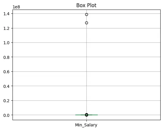
Winsorizing to Cap Salaries
Let us use Winsorizing to limit extreme values by replacing them with the nearest non-outlier value.
This argument specifies that 1% of the data from both ends (lower and upper) should be replaced.
Top 1% Outliers: Replaced with the value at the 99th percentile. Bottom 1% Outliers: Replaced with the value at the 1st percentile.
#Winsorizing to cap top 1% outliers
from scipy.stats import mstats
dfCopy['Min_Salary'] = mstats.winsorize(dfCopy['Min_Salary'], limits=[0.01, 0.01])  # Replace top and bottom 1%
dfCopy['Max_Salary'] = mstats.winsorize(dfCopy['Max_Salary'], limits=[0.01, 0.01])

# Let us plot graph again

print("Box Plot for Minimum Salary")
dfCopy.boxplot(column='Min_Salary')
plt.title('Box Plot')
plt.show()

print("Box Plot for Maxmium Salary")
dfCopy.boxplot(column='Max_Salary')
plt.title('Box Plot')
plt.show()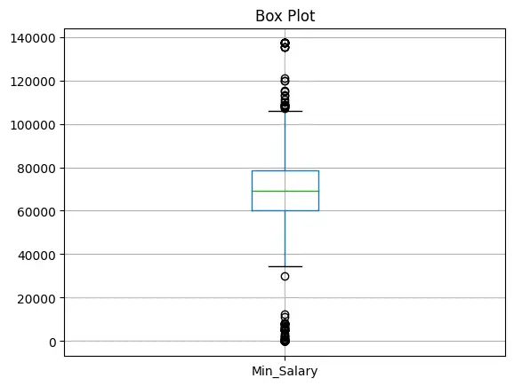
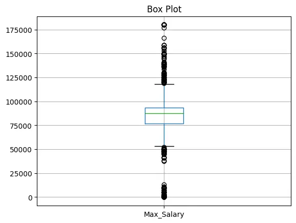
That is a big improvement, now since most lower bounds lie near 0, we can cap lower bound outliers to nearest minimum value. Upper bound values look fine.
# Cap or floor outliers in Min_Salary
dfCopy['Min_Salary'] = np.where(dfCopy['Min_Salary'] < lower_bound_min, lower_bound_min, dfCopy['Min_Salary'])
# dfCopy['Min_Salary'] = np.where(dfCopy['Min_Salary'] > upper_bound_min, upper_bound_min, dfCopy['Min_Salary'])

# Cap or floor outliers in Max_Salary
dfCopy['Max_Salary'] = np.where(dfCopy['Max_Salary'] < lower_bound_max, lower_bound_max, dfCopy['Max_Salary'])
# dfCopy['Max_Salary'] = np.where(dfCopy['Max_Salary'] > upper_bound_max, upper_bound_max, dfCopy['Max_Salary'])

# Display the DataFrame
print(dfCopy[['Min_Salary', 'Max_Salary']])
Let us check minimum and maximum values in Min_Salary & Max_Salary column.
new_minmin_salary = dfCopy['Min_Salary'].min()
new_minmax_salary = dfCopy['Min_Salary'].max()

new_maxmin_salary = dfCopy['Max_Salary'].min()
new_maxmax_salary = dfCopy['Max_Salary'].max()

print("Min Salary")
print(f"Minimum : {new_minmin_salary}")
print(f"Maximum : {new_minmax_salary}")
print("\n")
print("Max Salary")
print(f"Minimum : {new_maxmin_salary}")
print(f"Maximum : {new_maxmax_salary}")

# Output for above code

Min Salary
Minimum : 32250.0
Maximum : 137280.0


Max Salary
Minimum : 52100.0
Maximum : 180000.0
Looks better now, let us find average salary.
#Calcuate the Average Salary
def calculate_average(min_salary, max_salary):
    if min_salary is not None and max_salary is not None:
        return (min_salary + max_salary) / 2
    return None

dfCopy['Avg_Salary'] = dfCopy.apply(lambda row: calculate_average(row['Min_Salary'], row['Max_Salary']), axis=1)
We are done with cleaning our data, let us analyze column names and also rename for better readability.
dfCopy.isnull().sum()

# Output for NULL values

Position          0
Company           0
Skill             0
Salary            0
City              0
Province          0
Refined Title     0
Vector            0
Cluster           0
Job Roles         0
Seniority         0
Position Type     0
Work Type         0
Industry Type     0
Refined Salary    0
Min_Salary        0
Max_Salary        0
Avg_Salary        0
dtype: int64
Generating Output DataFrame 📤
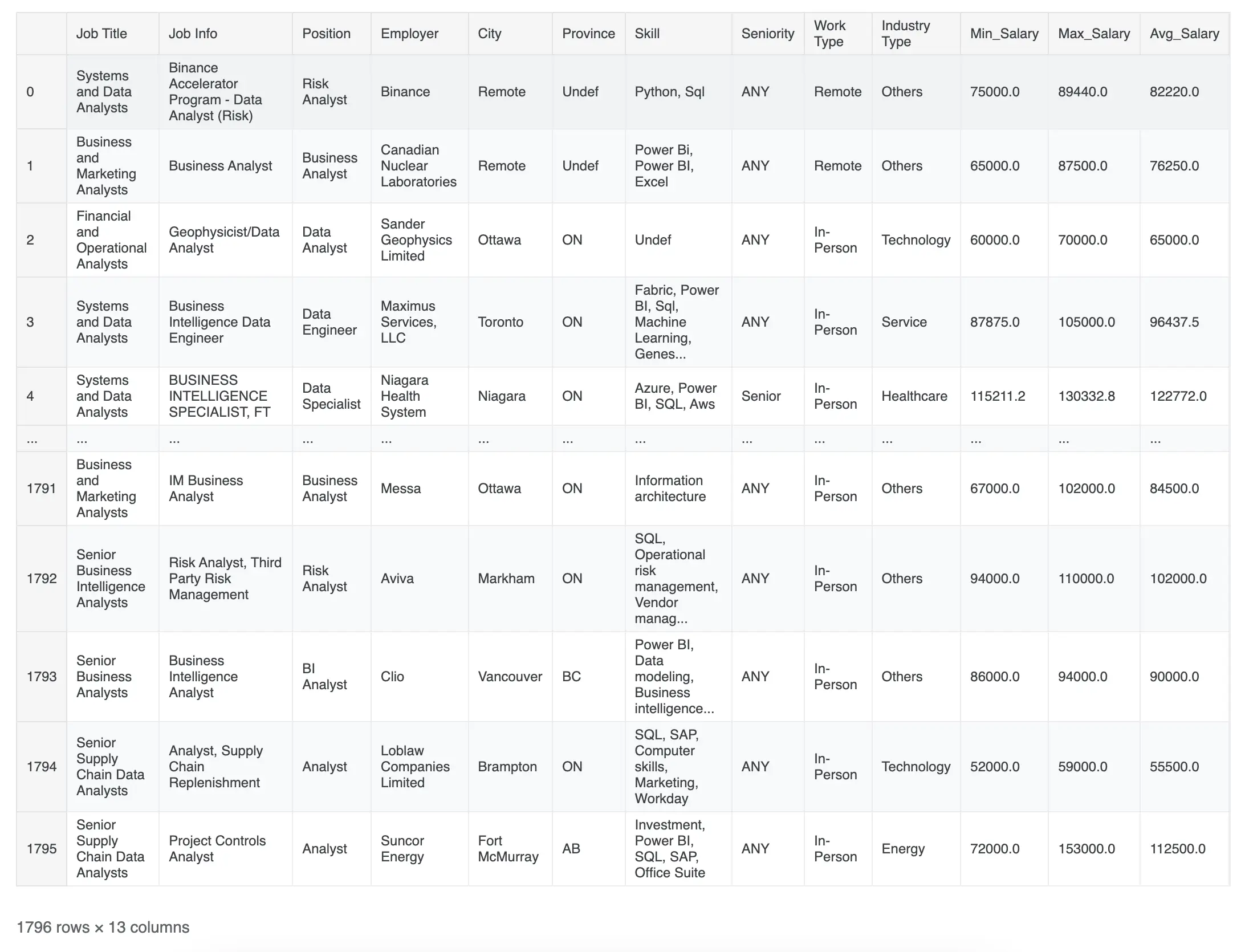
Let us rename some columns and output our cleaned dataset as a .csv file 📂.
# Create a new DataFrame with selected columns and rename columns
dFinal = dfCopy[['Job Roles','Position', 'Position Type','Company', 'City','Province','Skill','Seniority','Work Type','Industry Type','Min_Salary', 'Max_Salary', 'Avg_Salary']].rename(columns={
    'Company': 'Employer',
    'Job Roles': 'Job Title',
    'Position': 'Job Info',
    'Position Type':'Position',
})

# Printing our final dataframe
dFinal
Final Cleaned DatFrame Output -
Let us export our dataframe as a Comma Separated Values file 📂.
# Export df to CSV
dFinal.to_csv('Cleaned_Dataset.csv', index=False)
I hope you loved ❤️ the content. You can view this notebook live at Kaggle.
What's Next?
Next step is Data Exploration, and answering business problems. I've performed a thorough data visualization to answer my questions related to Data Analyst Job Trend in Canada. You can find more details in this article.